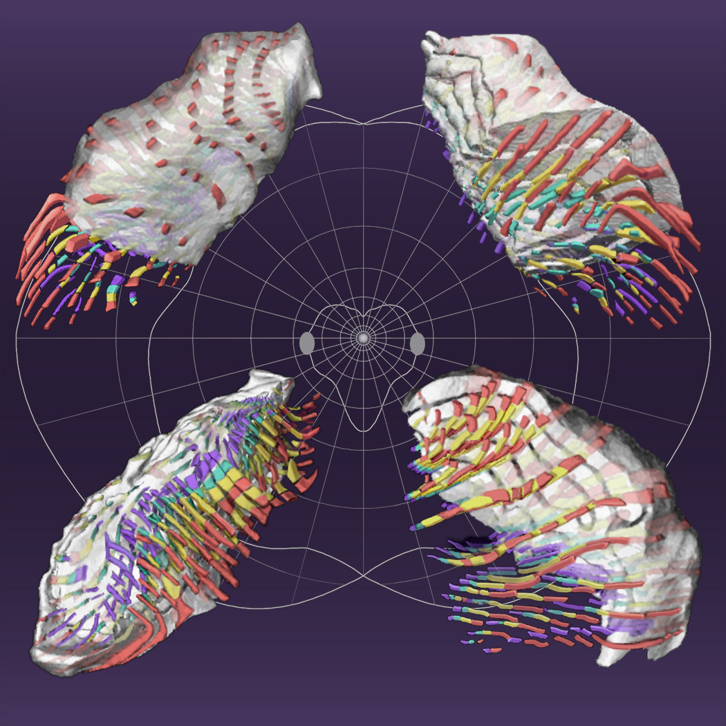
Atlas of a Rhesus Lateral Geniculate Nucleus (LGN)
|
Projection columns representing directions in visual space: red, contra-eye
parvo; yellow, ipsi-eye parvo; green, ipsi-eye magno; blue, contra-eye magno.
Columns are retinotopically located at intersections of the light grey
background polar grid (more clearly visible on the
high-resolution image): inclinations every
15°; eccentricities spanning roughly equal distances in the nucleus (0,
1.0, 1.9, 3.4, 6.3, 11.3, 19.2, 30.7, 46.6, and 67.6 degrees).
The heart-shaped central figure intersecting the oval blind spots separates
regions of visual space represented by six (central) and four (peripheral)
geniculate layers. Cut faces of semitransparent views pass though the blind
spot: upper panels show the 17° isoeccentricity surface; lower panels
show the minus 7° isoinclination surface. The posterior pole (foveal
representation) is in the uppermost part of each panel; the lower-left panel
shows the ventral surface. Projection columns are retouched to improve
clarity.
Made with the assistance of Janet Sinn-Hanlon of the Visualization, Media, and Imaging Laboratory
of the Beckman Institute for
Advanced Science and Technology, University
of Illinois at Urbana-Champaign.
|
This atlas was created by Ed Erwin,
Frank Baker, William Busen, and Joseph Malpeli for the
study described in Erwin et al., 1999, Relationship between laminar topology
and retinotopy in the rhesus lateral geniculate nucleus: results from a
functional atlas, Journal of Comparative Neurology, 407: 92-102, 1999.
with support from a grant from the National Eye Institute (NIH RO1 EY02695).
That paper describes the limitations of the atlas, and the user would be wise
to take note of these. The atlas provides only data files; software for
analysis or visualization must be obtained by the user. Three-dimensional
rendering of such large files requires fairly powerful computing resources,
but one can still obtain insightful views of the nucleus if the linear
resolution of the arrays is reduced by a factor of 2 or 3, thus reducing the
size of the data set by a factor of 8 or 27. The three-dimensional renderings
presented in Erwin et al. (1999) were generated with the Analyze® Biomedical
Imaging Application Package (Mayo Foundation); we have also viewed
two-dimensional cuts through the LGN with
Matlab.
The following text describes the format of the data files containing the atlas.
Good luck - Ed Erwin, Frank Baker, Bill Busen & Joe Malpeli
The first four data arrays described below have dimensionality 240 (medial-lateral) x 280 (dorsal-ventral) x 320 (anterior-posterior), with each voxel representing a 25 x 25 x 25 micron volume.
The first 240 entries represent a medial-lateral line of voxels, the next 240 entries represent an adjacent medial-lateral line of voxels in the same coronal plane, and so on (280 times) until that coronal plane is complete.
Then this sequence is repeated for the next coronal plane, and so on (320 times) until the volume is complete.
The Horsley-Clarke position of the origin of this coordinate system is 8.5 mm
lateral, -1.5 mm dorsal, and 3.5 mm anterior, with increasing array indices
corresponding to increasing distance in the lateral, dorsal and anterior
directions. These arrays are supplied in binary integer files (little-endian
format - low byte is least significant) without headers.
- ECC.DAT (43,008,000 bytes) is a three-dimensional array mapping
eccentricity. Eccentricity (rounded to the nearest 0.1°, then multiplied
by 10) is stored as 16-bit integers. Extralaminar space is coded 999. The
central 1° posed special problems in assigning
eccentricities. Available in PKZIP or UNIX Compress format.
- INCL.DAT (43,008,000 bytes) is a three-dimensional array mapping
inclination. Inclination (rounded to the nearest degree) is stored as 16-bit
signed integers. The two 90° sectors representing ipsilateral hemifield
are coded by assigning inclinations of -135° or +135° uniformly to the
lower and upper ipsilateral quadrants, respectively. Extralaminar space is
coded 999. Available in PKZIP or
UNIX Compress format.
- LAYERS.DAT (21,504,000 bytes) is a three-dimensional array mapping laminar
morphology. Layer type is stored as 8-bit integers: 1 = contra magno; 2 = ipsi
magno; 3 = ipsi parvo; 4 = contra parvo. Extralaminar space is coded zero.
Available in PKZIP or UNIX
Compress format.
- CELLS.DAT (43,008,000 bytes) is a three-dimensional array mapping cell
density. Cell density (cells/voxel multiplied by 1000) is stored as 16-bit
integers. CELLS.DAT is provided for convenience - it can be reproduced from
LAYERS.DAT and the cell density functions given later.
Available in PKZIP or UNIX
Compress format.
- FOVEOLA.DAT is an ASCII list of coordinates
(lateral, dorsal, anterior) of voxels making up the projection column of the
center of the fovea. These are array indices, not Horsley-Clarke coordinates.
To obtain the latter, multiply each coordinate by 0.025 mm and add the products
to the corresponding Horsley-Clarke coordinates of the lowest-valued corners
of the bit-mapped arrays. This column is narrower than the region coded 0 in
ECC.DAT because eccentricity values < 0.05° were rounded to 0 in ECC.DAT.
Note that visual space was mapped in spherical polar coordinates, the
coordinate system E, Figure 2 of Bishop et al., 1962 (J. Physiol. 163:
466-502). Retinotopy is mapped continuously across the LGN, spanning
interlaminar spaces and optic-disk gaps. It often extends slightly beyond
the outer borders of the LGN, to an extent that occasionally differs for
ECC.DAT and INCL.DAT.
The number of cells per voxel as functions of Horsley-Clark anterior position
is given below. These are equations of the curves shown in Figure 2 of Malpeli
et al. (1996, J. Comp. Neurol. 375: 363-377), except that the factor of
0.000625 (0.025²) has been incorporated because their figure gave
cells/mm² for a 25 micron-thick slab, instead of cells/voxel.
     magno:   cells / voxel =  0.000625 (ax^3 + bx^2 + cx + d), where
                    a = -3.6220071
                    b =  95.829137
                    c = -852.45404
                    d =  2732.8129
     parvo:    cells / voxel =  0.000625 (ax^6 + bx^5 + cx^4 + dx^3 + ex^2 + fx + g), where
                    a =  0.2893099
                    b = -14.997893
                    c =  317.08614
                    d = -3499.3549
                    e =  21249.945
                    f = -67304.569
                    g =  87499.769
Last modified: January 30, 2008